1. Sample Filtering and Quality Evaluation • utanos

Introduction

The utanos package begins with relative copy-number (rCN) call genomic data. It expects rCN data output from tools such as QDNASeq or WiseCondorX. This data consists of calls (a numeric value) for each ‘bin’ in the genome. A bin is an artificially defined partitioning of the genome into pieces of sufficient size to reasonably estimate a relative copy-number. For shallow sequencing this is needed because there is not sufficient depth present for base-pair level resolution.

Tabular long-format example:

chromosome   start     end sample    CN.call
<chr>        <int>   <int> <chr>       <dbl>
1           900001  950000 VOA14948A    1.00
1           950001 1000000 VOA14948A    1.00
1          1000001 1050000 VOA14948A    1.00
1          1050001 1100000 VOA14948A    1.00
1          1100001 1150000 VOA14948A    0.96
1          1150001 1200000 VOA14948A    0.96

Relative CN-callers such as QDNAseq sometimes have built-in QC functionality for filtering out bins. Most commonly this is for low-mappability or blacklist regions (see the paper for descriptions). Other CN-callers also can have whole-sample QC evaluation options though the vast majority of these tend to be very manual. They require the researcher to examine every individual sample. This vignette will cover how utanos can be used to do filtering and QC evaluation on an individual or group level.

I - Filtration

Often, in order to focus on the CN-aberrations of most interest, it is convenient to filter out more than just blacklist regions. What about centromeres? Telomeres? There are regions of the genome that are commonly copy-number aberrant in the background human population. Perhaps it would be nice to mask these too. Utanos clarifies the filtration process.

Note: Utanos comes with 2 tables of common variants (one for hg19 and the other hg38). They can be used to filter a dataset like so.

rcn.obj <- readRDS("~/Path_to_your_data/a_data_object_aligned_to_hg38.rds")
rcn.obj <- FilterCNs(cnobj = rcn.obj,
                     genome = "hg38",
                     minimum_overlap = 5000,
                     removebins = FALSE,
                     maskgaps = TRUE,
                     maskcomCNVs = TRUE)

Database of Genomic Variants (DGV)
The associated paper

But let’s break down this filtration step using a real example dataset. An accompanying data package to utanos is utanosmodellingdata found here. Clone that repo to somewhere convenient such as a common ‘repos’ folder on your machine and read in the sample data. It is human endometrial carcinoma sWGS data aligned to hg19.

> library(utanos)
> library(magrittr)
> rcn.obj <- readRDS("~/repos/utanosmodellingdata/sample_copynumber_data/sample_rcn_data.rds")
> rcn.obj <- FilterCNs(cnobj = rcn.obj,
                       genome = "hg19",
                       minimum_overlap = 5000,
                       removebins = FALSE,
                       maskgaps = TRUE,
                       maskcomCNVs = TRUE)
> featureData(rcn.obj)@data %>% head(5)
                chromosome  start    end     bases       gc mappability blacklist residual   use
1:1-30000                1      1  30000  66.66667 55.48500    12.39630  3.263333      NaN FALSE
1:30001-60000            1  30001  60000 100.00000 39.75667    28.22070  0.000000      NaN FALSE
1:60001-90000            1  60001  90000 100.00000 36.13000    27.47780  0.000000      NaN FALSE
1:90001-120000           1  90001 120000 100.00000 39.61667     9.05091  0.000000      NaN FALSE
1:120001-150000          1 120001 150000 100.00000 46.52333     7.33796  0.000000      NaN FALSE
                centro.telo.mask comCNV.mask
1:1-30000                  FALSE       FALSE
1:30001-60000               TRUE       FALSE
1:60001-90000               TRUE       FALSE
1:90001-120000              TRUE       FALSE
1:120001-150000             TRUE       FALSE

This sample data had relative copy-numbers called by QDNAseq. The ‘use’ column in the S4 object indicates bins QDNAseq determines to be useable. The bins with ‘FALSE’ are not. For more details on QDNAseq and its methods see the bioconductor vignette here. The FilterCNs utanos function adds another two columns to the featureData table because the maskgaps and maskcomCNVs parameters were set to TRUE. The use, centro.telo.mask, and comCNV.mask columns we will refer to as ‘masks’, as if you subset by these columns you essentially mask them from downstream analysis.
A final note on the FilterCNs function: using the filter_by parameter a user can provide their own regions by which to create a mask or filter the QDNAseq copy-number object. Just pass a dataframe with the locations, one location per row, to the filter_by parameter. Using the maskname parameter the user can set the name for the mask. The maskname parameter expects a character string.

Next, we can visualize the masks using the CNSegmentsPlot function.

> a <- CNSegmentsPlot(rcn.obj,
                      sample = "CC-CHM-1341",
                      highlight_masks = c('comCNV.mask'),
                      point_size = 0.5,
                      dolog2 = TRUE, 
                      def_point_colour = 'grey')
> a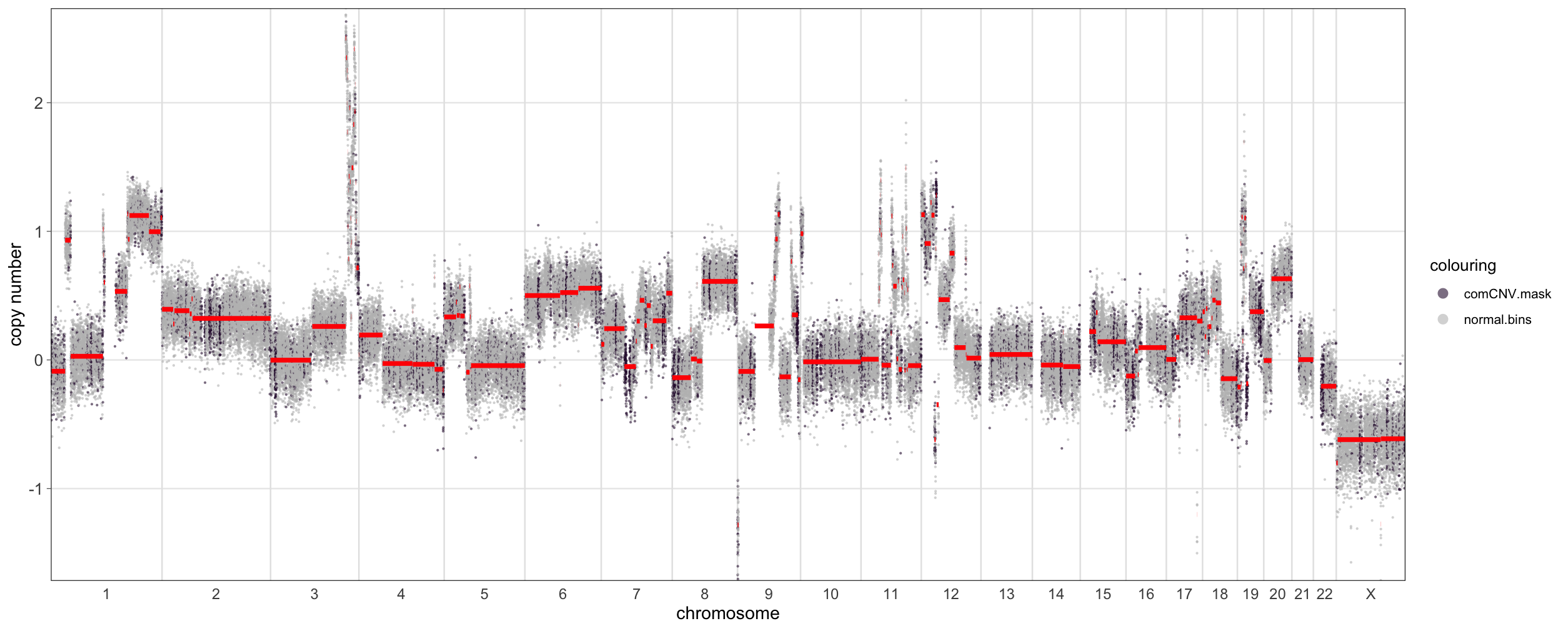

Clearly visible in the plot is that several of the regions that are commonly copy-number variant in humans coincide with a copy-number/segmentation change. Depending on the user’s specific use case these regions may or may not be worth excluding.
Note: The dolog2 parameter was set to TRUE in this call so we see the copy-number calls and segments log2 transformed and so centered about 0. See the documentation for that function for more details.

II - Sample Quality Evaluation

Shallowly sequenced whole genome data involves copy-number calling in two stages: relative copy-calling (via tools such as QDNASeq and WiseCondorX) and then absolute copy number calling which is run on the relative calls (via tools like rascal). Naturally, the accuracy of the inferences that can be made in downstream analysis depend heavily on the accuracy of the copy number calls inferred. However, for large projects it is an intensive demand to manually evaluate the quality of hundreds to thousands of samples. This is another the niche that Utanos fills.

Use the GetSampleQualityDecision function to get quality calls for each sample in your dataset. The QualityPlot function can then be used to visualize the samples that fall outside the thresholds.

> qc_decisions <- GetSampleQualityDecision(rcn.obj)
> qc_plot <- QualityPlot(qc_decisions)
> qc_decisions %>% head(5)
       sample seg_counts  median_sd decision seg_cut    med_cut
1 CC-CHM-1341        204 0.07696209     High   620.3 0.09096386
2 CC-CHM-1347        695 0.07137276      Low   620.3 0.09096386
3 CC-CHM-1353        235 0.06784682     High   620.3 0.09096386
4 CC-CHM-1355        240 0.07509611     High   620.3 0.09096386
5 CC-CHM-1361        529 0.07547814     High   620.3 0.09096386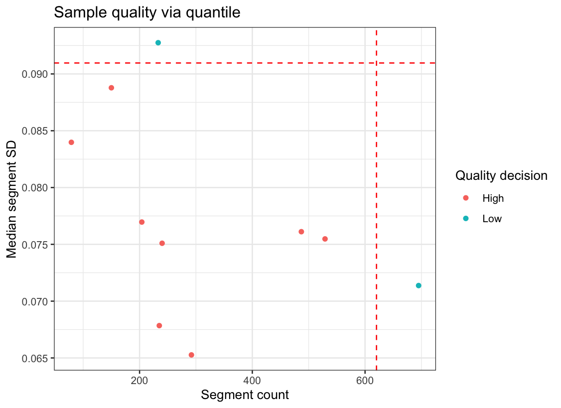

> qc_plot

The default behaviour of this function is make a sample-wise decision based on thresholds for the median segment standard deviation and the total segment count.

II.1 - About the metrics: Median segment variance and segment count

The segment variance is calculated as the sample variance per segment, i.e the variance between the $log_2$ ratios of each bin in each segment. The observed median segment variance then is a sample-wise measure for noise, which is defined as the median of a set of variances.

The segment count is simply the number of distinct segments found in the sample. In poor quality samples over-segementation is a frequent indicator.

The strategy with this quality evaluation technique is to consider both of these metrics in tandem. To work through the intuition, consider the following two copy-number profiles:

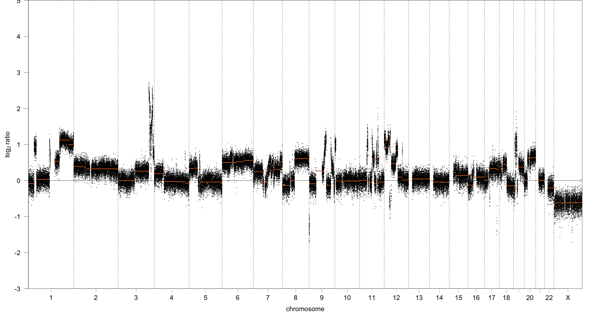
Sample 1: Good quality copy-number profile

Sample 2: Poorer quality copy number profile

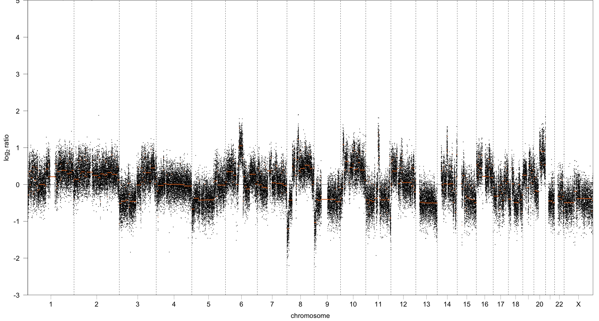
The key aspects that differ between the two profiles are: the number of segments, the length of segments, and the variance within each segment of the $log_2$ ratios, i.e we see the copy number ratios more tightly clustered around the orange line for sample 1 compared to sample 2.

III - Possible future additions and ideas: The copy-number profile abnormality score penalty

This is a metric to distinguish abnormal from healthy copy number profiles. The score quantifies the deviation of segments from the normal diploid state at the sample-level. The copy-number profile abnormality score can be expressed as follows:

$CPA \ = \ \frac{\Sigma^{n}_{i=1} (|Z_{segment_i}|* l_{segment_i})}{n}$

Here, $Z_{segment_i}$ represents the $Z$ -score of the segment $i$ . $l_{segment}$ represents the length of the segment and $n$ represents the number of segments.
The average segment length can be represented as follows:

$\frac{\Sigma^{n}_{i=1}l_{segment_i}}{n}$

This term functions as a penalty term for sample quality, as short segments are generally observed in bad quality or truly highly aberrant samples. Thus, calculating this penalty in addition to other metrics could be very informative. A very important note is that alone this metric would be problematic. Copy-number aberrant is an expected state when the biology of the sample truly is chromosomal aberrations. This metric in tandem with others would seek to find aberration where none should be present.

Thus, a future workflow could be a classifier (which would be trained on our test set) with the features being the segment sizes, median segment variances, the Lilliefor normality statistic, read length, coverage etc.